It is two days before your taxes are due. You have a big box of receipts, pay stubs, invoices and forms. And you don't want to pay another late filing fee after the deadline has passed. How it works?
You could spend hundreds or thousands of dollars on an emergency tax session with an accountant. Or you can use the power of Excel to get everything in order.
Use of VLOOKUP for tax tables
The VLOOKUP function has a very useful optional operator. If this operator is set to FALSE, the function will return an error if the value you are looking for is not displayed. However, if set to TRUE, the next lower number will be returned. This is perfect for control tables. Here is a hypothetical control table:
Let's say you need tax information for three different people. This means that you need to do the same calculation for three different incomes. Use VLOOKUP to speed up the process. Here is the syntax we will use:
= VLOOKUP (A2, A1: B6, 2, TRUE)
A2 is the income amount, A1: B6 is the cell range that contains the tax rates, 2 specifies that values from the second column should be returned, and TRUE tells the function to round down if no exact values are found Game.
Here's what happens when we run it on cells that contain 37.000, 44.000 and 68.000 US dollars for income values included:
As you can see, the correct tax rate was returned for all three of them. Multiplying the tax rate by the total income is simple and gives you the amount of tax you need to pay for each amount. It's important to remember that VLOOKUP runs round low If it doesn't find the exact value, it searches. So when you set up a table like the one shown here, you need to specify the maximum values from the ranges that apply, not the minimum values.
VLOOKUP can be extremely powerful. Read Ryan's article about Excel formulas that do crazy things. 3 Crazy Excel Formulas That Do Amazing Things 3 Crazy Excel Formulas That Do Amazing Things Conditional formatting formulas in Microsoft Excel can do wonderful things. Here are some great tricks for Excel formula productivity. Read more to find out what it is capable of doing!
The IF function for multiple thresholds
Some tax credits depend on how much money you earned. In this case, you nest IF statements and other boolean operators. Mini Excel tutorial: use Boolean logic to handle complex data. Mini Excel tutorial: use Boolean logic to process complex data. The logical operators IF, NOT, AND, and OR can help you get from Excel novice to power user. We explain the basics of each function and show how you can use them for maximum results. With Read More you can easily find out how much you can reclaim. Using the Earned Income Credit (EIC), we create an example. I've highlighted the relevant part of the EIC table here (the four columns on the right are for married couples filing jointly and the four on their left are for single filters):
Let's write a statement that determines how much we can reclaim through EIC:
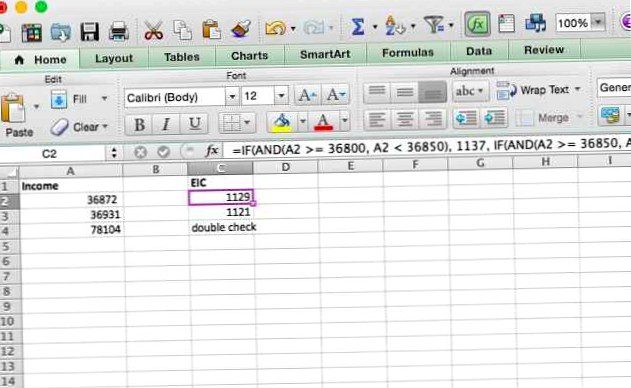
= IF (AND (A2> = 36800, A2) < 36850), 1137, IF(AND(A2 >= 36850, A2 < 36900), 1129, IF(AND(A2 >= 36900, A2 < 36950), 1121, IF(AND(A2 >= 36950, A2 < 37000), 1113, "double check"))))
Let's break this down a bit. We'll just take a single statement that looks like this:
= IF (AND (A2> = 36800, A2) < 36850), 1137, 0)
Excel looks at the AND statement first. If both logical operators in the AND statement are true, it returns TRUE and then returns the [value_if_true] argument, which in this case is 1137. If the AND statement returns false (z. B. A2 = 34.870), this will The function returns the [value_if_false] argument, which in this case is 0.
In our current example, we used a different IF statement for [value_if_false], which allows Excel to execute IF statements until one of them is true. If your income passes through the final statement without being in one of these ranges, the string "check" is returned to remind you that something is going on. Here's what it looks like in Excel:
In many cases you can use VLOOKUP to speed up this process. However, understanding nested IF statements can be helpful in many situations you may encounter. And if you do this frequently, you can create a template for a financial spreadsheet. 15 Helpful Spreadsheet Templates to Manage Your Finances 15 Helpful Spreadsheet Templates to Manage Your Finances Always keep track of your financial health. These free spreadsheet templates are just the tools you need to manage your money. Read more with these functions built in for reuse.
Calculating the interest paid with ISPMT
Knowing how much interest you paid on a loan can be valuable on your taxes. However, if your bank or lender does not give you this information, it can be difficult to find out. If you provide ISPMT with some information, this will calculate for you. Here's the syntax:
= ISPMT ([rate], [period], [nper], [value])
[Interest rate] is the interest rate per payment period, [period] is the period for which the interest is calculated (z. B. if you have just made your third payment, this is 3). [nper] is the number of payment periods you need to pay off the loan. [value] is the value of the loan.
Let's say you have a mortgage in the amount of 250.000 US dollars with an annual interest rate of 5%, and you pay it off in 20 years. This is how we calculate how much you paid after the first year:
= ISPMT (0.05, 1, 20, 250000)
If you run this in Excel, you will get a result of 11.$875 (as you can see, I set this up as a table and selected the values there)..
If you use this for monthly payments, you need to convert the annual interest rate to a monthly interest rate. When determining the amount of interest due after the third month of a one-year loan of 10.000 USD and an interest rate of 7% was paid, for example, the following formula would be used:
= ISPMT ((. 7/12), 3, 12, 10000)
Conversion of nominal interest rates into annual interest rates with EFFECT
Calculating the actual annual interest rate of a loan is a great financial skill. If you get a nominal interest rate that compounds several times during the year, it can be difficult to know exactly what you will pay. EFFECT will tell you.
= EFFECT ([nominal_rate], [nper])
[nominal_rate] is the nominal interest rate, and [nper] is the number used to compound the interest rate during the year. We'll use the example of a loan with a nominal interest rate of 7.5%, compounded quarterly.
= EFFECT (0.075, 4)
Excel gives us the effective annual interest rate of 7.71%. This information can be used with a number of other functions that use interest rates to determine how much you paid or how much you owe. It can also be useful to set up a personal budget using Excel. Create a personal budget in Excel in 4 easy steps. Create a personal budget in 4 simple steps. Have so much debt that it will take decades to pay off? It's time to create a budget and apply a few Excel tricks that will help you pay off your debt faster. Read more .
Depreciate assets with DB
Excel contains a number of different depreciation functions. However, we consider DB, the fixed descending balance method. Here's the syntax:
= DB ([cost], [salvage], [life], [period])
The argument [cost] represents the initial cost of the asset, [salvage] is the value of the asset at the end of the amortization period, [life] is the number of periods over which the asset declines, and [period] is the period number for which you want to obtain information.
Interpreting the results of the DB statement can be a little complicated, so we'll look at a range of data. We take an asset value with an initial cost of 45.USD 000 on, which over the course of eight years amounts to 12.000 USD loses. Here's the formula:
= DB (45000, 12000, 8, 1)
I'm going to run this formula eight times, so the last argument will be 1, 2, 3, 4, 5, 6, 7, and 8 on consecutive lines. Here's what happens when we do:
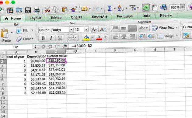
The number in the depreciation column is the amount that was lost. To see the value of the investment at the end of the year, you need to subtract the number in the Depreciation column from the value of the investment at the beginning of that year. To get the value at the end of the first year, we subtract $6.840 from $ 45.000 off and receive $ 38.160. To get the value at the end of the second year, we subtract 5.$800.32 from 38.160 $ and receive 32.359,68 $. And so on.
Excel for taxes
These five features are among the many available and should help you harness the power of Excel to get your taxes done. If you are not an Excel fan, you can also use the money management tools in Google Drive 10. Money management tools in Google Drive you should use today. 10 Money Management Tools in Google Drive You Should Use Today. The problem with the money is that you do not manage it, you end up without. How about some useful money management tools to help you get started with your Google Drive account? Read more . And don't forget that there are many other great resources, including some useful IRS 7 IRS website tools that could save you time and money. 7 IRS website tools that could save you time and money a few online IRS tools for U.S. citizens who diligently file their taxes. You make your work much easier. Don't give up yet. Read more and a variety of downloadable Excel programs. Top 3 websites to download useful free Excel programs Top 3 websites to download useful free Excel programs Continue reading .
If you use Excel to manage your taxes, please share your tips below! We'd love to hear which features you use most often. If you want to use Excel for taxes and aren't sure how to do something, leave a comment with a question and we'll do our best to respond.